A Levey-Jennings chart tells you that something moved. It doesn’t tell you why. The dots are a symptom, and the job of a scientist is to work back from the pattern to the cause.
This article picks up where How to Read a Levey-Jennings Chart left off. We’ll look at the two kinds of error behind every wobble, where the mean and SD on your chart come from, how reagents and instruments drift, what calibration does and doesn’t fix, the reasoning behind the Westgard rules, and a sensible order of checks when QC fails. The pace is a little slower than last time, because the rules are easier to apply when we understand what they detect.
1. Two ways to be wrong: random and systematic error
Every measurement error can be split into two kinds, and almost everything in QC follows from the difference between them.
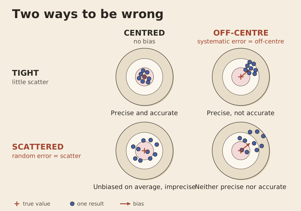
Random error makes repeated measurements scatter. Repeat the same measurement and you get a spread of results around some value. We call that scatter imprecision, and we measure it with the standard deviation (SD) or the coefficient of variation (%CV). Systematic error pushes results consistently in one direction. How far the average sits from the true value is the bias.
Total analytical error is what a single result actually carries: the bias plus whatever random scatter happens to land on that result, acting together. Don’t confuse it with allowable total error (TEa), which isn’t a measurement at all. It’s a goal: how much error a result can carry before it starts to mislead a clinician. Much of QC comes down to one question: is the error you have comfortably smaller than the error you can afford?
A word on %CV. The SD is in the units of the test, so an SD of 2 means something very different when the mean is 10 than when it is 100. The %CV fixes that by expressing the SD as a percentage of the mean. It’s the everyday shorthand for relative imprecision. It lets you compare two assays, two control levels or two analysers on the same scale, and it’s a common way to summarise imprecision over time.
%CV = (SD ÷ mean) × 100
The same SD gives a very different CV at different levels:
| Mean | SD | Calculation | %CV |
|---|---|---|---|
| 10 | 2 | 2 ÷ 10 × 100 | 20% |
| 100 | 2 | 2 ÷ 100 × 100 | 2% |
The CV also depends on the level of the control, so when you quote one, say which control it belongs to. Here is a hypothetical example for an ALT control (our own illustration, not real data):
| Control | Mean (U/L) | SD (U/L) | Calculation | %CV |
|---|---|---|---|---|
| Low | 30 | 0.9 | 0.9 ÷ 30 × 100 | 3.0% |
| High | 240 | 1.5 | 1.5 ÷ 240 × 100 | 0.63% |
The SD rose only a little while the mean rose eightfold, so the CV fell sharply. The low control looks proportionally the worst even though its absolute scatter is smaller. For QC, use the CV from your own long-term data, which includes day-to-day and calibration-to-calibration variation, rather than a short within-run figure, which understates what your chart will see. A quick repeatability experiment (one run, one reagent pack, one calibration) only sees the scatter within that run. Over weeks, the chart also sees new packs, calibrations, operators and maintenance. In one manufacturer’s ALT precision study, a control near 30 U/L had a within-run SD of 0.5 U/L but a 20-day SD of 0.9 U/L, and that was with a single reagent lot and a single analyser. Limits built from the short figure would flag perfectly ordinary days.
Systematic error comes in two flavours:
- Constant error is the same size at every concentration, for example every result reading 10 units too high. Interference and a mis-set zero point are classic causes.
- Proportional error grows with concentration, for example every result reading 10% too high. A wrongly assigned calibrator value is a classic cause.
What each error does to the SD and %CV. Take a control with a mean of 100 and an SD of 3 (hypothetical numbers):
| Situation | Mean | SD | %CV | What happens |
|---|---|---|---|---|
| Baseline | 100 | 3.0 | 3.0% | Working as expected. |
| More random error | 100 | 6.0 | 6.0% | The spread doubles. SD and %CV double with it. |
| Constant error (+10) | 110 | 3.0 | 2.7% | The mean moves. The SD is unchanged and the %CV barely changes. |
| Proportional error (+10%) | 110 | 3.3 | 3.0% | The mean and SD both rise by 10%. The %CV is unchanged. |
Random error shows up in the SD and %CV. Systematic error shows up as a moved mean, and a %CV that looks fine can sit on top of a badly biased result. That is why the %CV tells you about imprecision and not about trueness, and why we watch the mean as well.
On a daily QC chart, these errors show up as patterns:
- Scatter means the points are spreading wider than usual. That suggests the SD has grown, which points to worsening imprecision (random error).
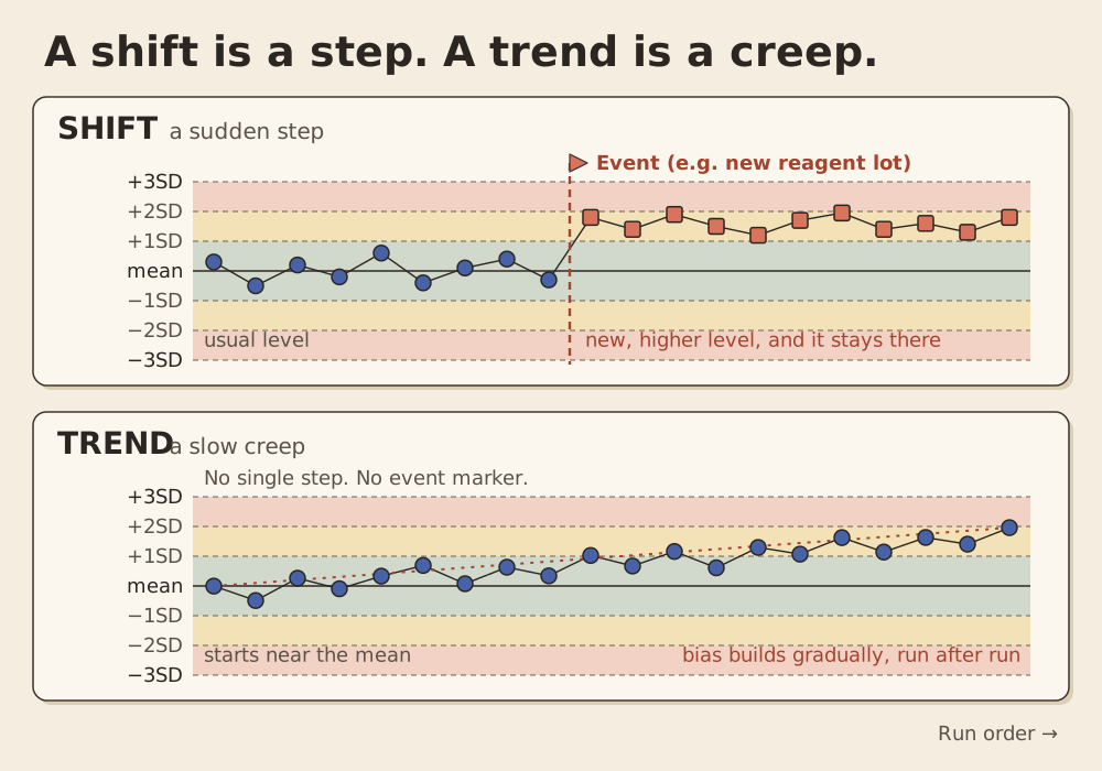
- A shift is a sudden step to a new level. That suggests a step in bias.
- A trend is a slow creep in one direction. That suggests bias building gradually.
If you look at two control levels, they give you a clue about constant versus proportional error. A constant error moves both levels by the same amount. A proportional error moves the high control further than the low one. Plotting both levels in SD units (how many SDs each result sits from its own mean) lets you compare them side by side, though an equal absolute shift won’t look equal if the two levels have different SDs.
One caution. The link between a pattern and a cause is a clue, not a diagnosis. A shift tells us the QC results have moved away from their usual baseline. Sometimes the same change affects patient results. Other times, the change is limited to the control material itself. A big enough shift can trip a rule built for random error, and a random blow-out can trip a rule built for systematic error.1
2. Where the mean and SD come from
The centre line and limits on your chart are only as good as the data behind them. This is the least glamorous part of QC and one of the most important, because every rule assumes the mean and SD describe your system when it’s working properly. So the data should come from a stable period that looks like ordinary running, with the usual operators, reagent packs, calibrations and maintenance in it.
How much data? Recommendations differ in their starting requirements. Here is what several of the guidelines say:
| Source | Guidance |
|---|---|
| Westgard2 | At least 20 measurements over at least 10 working days, preferably 20. Too short a period underestimates the SD. |
| Bio-Rad QCNet (summarising CLSI C24)3,4 | At least 20 measurements on 20 separate days for a new control product. A shortcut such as 4 a day for 5 days gives provisional values only. |
| Australasian Association of Clinical Biochemists (AACB) workshop paper5 | As few as 20 points over at least 20 days to start, a review at 60 points, and 60 to 80 points per level for a reliable SD. |
Where they agree: 20 is a starting point, not a finish line. Early numbers are provisional, and the SD especially. If you pull it from five good days you will probably underestimate it, because you haven’t yet seen a new operator, a maintenance cycle or a new reagent pack. A chart with an SD that’s too tight will cry wolf. A chart with an SD that’s too loose will stay silent when it shouldn’t.
Own data or the manufacturer’s range? Use your own once you have enough of it. While your own numbers are still provisional, the manufacturer’s insert range and any peer-group data are a useful yardstick to check them against.3 One limit of local statistics is that they describe stability, not trueness: a lab can have a stable mean while its patient results are biased, so your own mean and SD still need to be judged against appropriate analytical performance goals. Internal QC tells you whether performance has moved away from its own baseline. Whether that baseline is right is a job for method comparisons, suitable reference materials and external quality assessment (EQA). Manufacturers may set ranges wide enough to cover most systems in the field, so a range can be much wider than appropriate for QC within a single laboratory.6 Manufacturer ranges are often indicative of about ±3 SD.5 The ranges printed in a control’s package insert are for guidance only. The manufacturer’s range is a good place to start and a poor place to stay.
Keeping it honest. A few habits protect the numbers:
- When you calculate the mean and SD, leave out the control results from runs that were rejected for an assignable fault in that assay. The whole run for that assay is suspect, not just the point that failed. Leaving a result out of the baseline calculation isn’t deleting it: keep every result in the audit record. And not every statistical rejection proves a fault, so judge each one on its merits.
- Review the running mean and SD against your targets at about one month, then at least monthly.5 Keep an eye on the %CV as well as the mean: a CV that creeps up over several months can mean the imprecision is changing, even before many points breach their limits.
- Change a target only deliberately, by an authorised person, as a last resort. Moving the target so the dots fit defeats the purpose.
- When a new lot starts, work out whether any shift is confined to the QC material (a matrix effect, called non-commutability) or shows up in patient samples too. If it’s QC-only, a new target mean is often justified.
3. Drift: when reagents and instruments wander
Things in a lab have a clock on them. Reagents deteriorate. Lamps and detectors age. Temperatures wander. None of this announces itself, and not every developing problem trips an analyser alarm. It shows up as a slow change in your points.
Typical contributors are:
- Reagent deterioration. It may show up as a calibration error or a control falling outside its range. On-board stability varies a lot between assays, from days to weeks.
- Instrument components. Detector drift, lamp integrity, probe and syringe performance, mixing, and reaction temperature.
- Water and environment. Purified water outside its specification, and ambient or reaction-chamber temperature.
- Control material. Material used past its open-vial stability, or stored badly, deteriorates and sends you chasing a fault that isn’t in the analyser.
- Lot changes. A new reagent or calibrator lot can move the whole chart in one step.7
Drift is real, but how fast it happens varies between platforms and assays.
What it looks like. As a rough guide, gradual deterioration tends to show as a trend, and an event (a new lot, a maintenance step, a calibration) tends to show as a shift. That’s a tendency, not a law: a shift or a trend is a clue that tells you where to start looking, not a diagnosis. Widening scatter is the third pattern, and it’s the easiest one to over-read: a handful of points can look noisy by chance. If the chart looks wider, check whether the SD or %CV of recent results has actually risen before calling it worse imprecision.
In the conventional Westgard rules, 4-1s and 10x are rejection rules. On very stable systems, some labs choose to use them as warnings instead, prompting action such as maintenance before a rejection rule fires.6 That’s an optional local adaptation, not part of the standard rule set, so a lab that does it should decide it deliberately and write it down.
4. Calibration: what it fixes and what it doesn’t
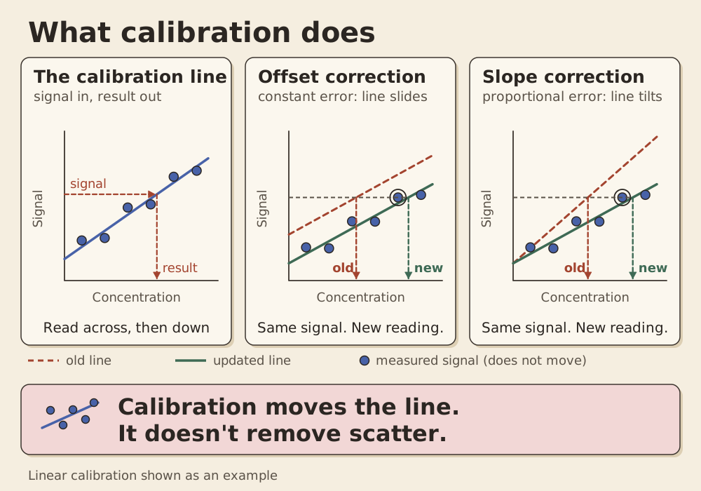
Calibration teaches the analyser how to turn a measured signal into a result. It uses calibrators with assigned values to establish that relationship. Sometimes it’s a straight line; other times it’s a curve. In effect, it’s designed to compensate for bias in the method.8
So recalibration can correct certain types of bias. Specifically, it re-anchors the signal-to-result relationship, which makes it good at correcting a consistent offset or a slow change in slope. But it can’t fix every problem, and a fresh calibration doesn’t guarantee accurate results.
It doesn’t fix:
- Imprecision. If results are scattering because of unstable pipetting or inconsistent reagent delivery, recalibrating won’t solve the underlying issue.
- A faulty part or reagent. A failing lamp or a blocked probe is still failing.
- Non-commutable QC material. If QC material behaves differently from patient samples, adjusting the calibration just to make it recover its target can move your patient results the wrong way.
- Interference in the sample.
The catch is that if a problem is unresolved, recalibration can compensate for it and hide it. QC looks fine straight afterwards, and the cause is still there.8 So the practical advice is to investigate before recalibrating.
How often? There’s no universal answer. Calibration intervals and recalibration triggers are set by the manufacturer for each assay and platform, and they vary widely, from every day to a month or more. Recalibration may also be required after a reagent lot change, after certain maintenance, or when QC falls outside acceptable limits. Follow the instructions for your own assay and platform. Calibration stability isn’t the same thing as how long the reagent lasts on the analyser.
When recalibration is appropriate. Manufacturers generally say recalibration may be necessary when QC falls outside acceptable limits, while professional guidance advises against it without a good reason.5 These aren’t actually in conflict. Follow the manufacturer’s instructions, but treat recalibration as the outcome of an investigation that points to calibration, not as the first move.
A subtle point. Calibration is itself a measurement. Different assays use different calibration procedures, with different numbers of calibrators and replicates, but every calibration carries its own measurement variation.9 If the variation between calibrations is large compared with the variation within one, the chart can step after each calibration. The rules that hunt for small, persistent shifts (2-2s, 4-1s and 10x) can then reject runs that may be fine.10 That doesn’t make a post-calibration shift acceptable by default, so it still needs checking before it’s dismissed.
5. The Westgard rules, as logic
The Westgard rules are often taught as a list to memorise. They make more sense as a design problem: how do you catch real errors without stopping the lab for false alarms?
A single wide limit, like 1-3s, rarely rejects a good run, but it has limited sensitivity to a small shift. A single tight limit, like 1-2s, notices more, but if you used it as a rejection rule, it would reject about 8.9% of perfectly good runs with two controls, 13.0% with three and 17.0% with four. (That’s our own arithmetic, assuming independent, normally distributed results and correctly set limits.) It’s the same trade-off as sensitivity and specificity in a diagnostic test. The usual design goals are high error detection, around 90% or more for a clinically important error of a specified size, and low false rejection, no more than about 5%.11 Those are targets for designing a QC procedure, not guarantees of how it will perform.
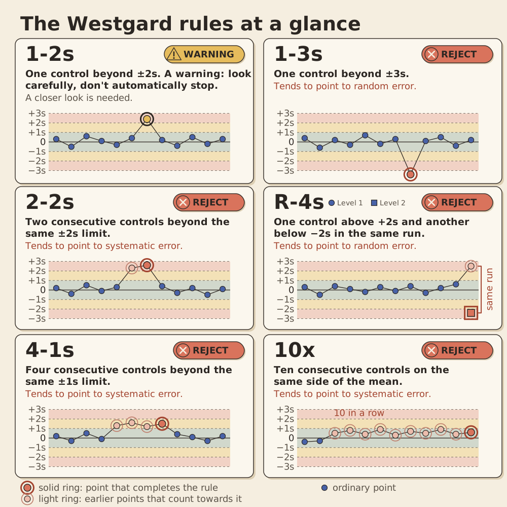
The multirule idea is to combine several rules so each covers another’s blind spot. A rule violation is a statistical pattern, not a confirmed cause, so read the last column below as “where to start looking”.
| Rule | Reads as | Tends to point to |
|---|---|---|
| 1-2s | One control beyond ±2s. A warning: look carefully, don’t automatically stop. | (needs a closer look) |
| 1-3s | One control beyond ±3s. Reject. | Random error, though a big shift can trip it |
| 2-2s | Two consecutive controls beyond the same ±2s limit. Reject. | Systematic error |
| R-4s | Two controls in the same run on opposite sides: one above +2s, the other below −2s. Reject. | Random error (read within a run) |
| 4-1s | Four consecutive controls beyond the same ±1s limit. Reject. | Systematic error |
| 10x | Ten consecutive controls on the same side of the mean. Reject. | Systematic error |
Each control level is judged against its own mean and SD. Some rules (2-2s, 4-1s and 10x) can be applied across control levels or across consecutive runs as well as within a run, while R-4s applies only within a single run.11
Classic versus modern. In the original procedure,16 1-2s was a gate: only if a result broke it did you check the other rules. That was to keep manual checking manageable. With computers doing the checking, there’s no need to apply the 1-2s rule at all,6,11 and the Sigma Rules (2014) drop it.12 “Westgard rules” also aren’t one fixed set. The original multirule is one example of a multirule procedure, and labs choose their own.
Sigma choosing the rules. The sigma metric is (allowable total error − |bias|) / %CV, all in percent, where |bias| is the size of the bias ignoring its sign.5 As a constructed example: if the allowable error is 10%, bias is 2% and the CV is 2%, sigma is (10 − 2) / 2 = 4. (Those numbers are invented to show the arithmetic.) Better-performing methods generally allow simpler QC, while less capable methods may need more rules, more control measurements or more frequent monitoring. Roughly, with two control levels, a 6-sigma method can get by with 1-3s alone, 5-sigma adds 2-2s and R-4s, and 4-sigma adds 4-1s, which needs four control results per decision (four in one run, or two in each of two runs). Methods below 4 sigma add an 8x rule and more control measurements again. The cut-offs differ slightly between published schemes,5,12 and the answer depends on which quality goal you choose for allowable error, and goals vary.
The Australian picture. Accredited laboratories work to ISO 15189 as applied by NATA. NATA’s assessment worksheet for clause 7.3.7.2 asks for QC at a frequency based on method stability and the risk of harm from a wrong result, defined acceptance criteria, data that make trends and shifts detectable, and no release of results when QC fails.13,14 Neither it nor the application document names “Westgard rules” or prescribes a rule set. The rule set is the laboratory’s decision, informed by Westgard and by AACB harmonisation advice.
The AACB workshop paper is also sceptical of rules that need several results from the same control level, and prefers running QC more often to running more replicates.5 That sits uneasily with classic Westgard teaching, and it’s a view rather than a regulation. Combine it with the calibration point above, and you can see why the rules you pick should depend on your system, not on tradition.
6. When QC fails: a sensible order of checks
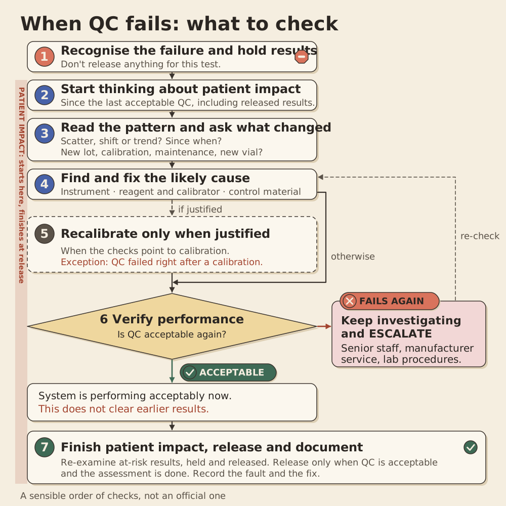
There’s no single official troubleshooting sequence. What follows draws on published checklists and Westgard’s protocol, so treat it as “a sensible order”, not “the rule”.1,5,15
- Recognise the failure and hold results. Hold patient results for the affected test. Don’t release anything while QC is failing.13
- Start thinking about patient impact straight away. Note when QC was last acceptable. Every result examined since then, including anything already released, may be affected. You’ll finish this assessment at the end, but don’t postpone starting it.
- Read the pattern and ask what changed. Look at this analyte’s chart. Is it scatter, a shift or a trend, and when did it start? Look at other analytes too. A problem across several tests points to something shared, like the water, the temperature or the control material. Then check events since the last good QC: maintenance, a new reagent pack or lot, a calibration, a new vial of control.
- Find and fix the likely cause. Work through the usual suspects:
- The instrument: flags, maintenance up to date, probes, lamps, cuvettes, water bath, power and temperature.
- The reagent and calibrator: correct reagent, enough volume, within expiry and on-board stability, calibrator values, lot, preparation and storage.
- The control material: out of date, open too long, or made up wrongly?
- Recalibrate only when justified. That means the earlier checks point to calibration. The exception is QC failing straight after a calibration, when the calibration is the first suspect.
- Verify that performance is acceptable again. Run QC again. If it’s acceptable, that’s evidence the system is performing acceptably now. That doesn’t show the original failure was harmless, and it doesn’t clear results from before. If it fails again, keep investigating, and escalate (senior staff, the manufacturer’s service, your lab’s procedures) rather than repeating indefinitely.
- Finish the patient-impact assessment, release, and document. Re-examine results from the at-risk window where a clinically significant error may have occurred, as your lab’s procedure requires.13 One published approach, from an Australasian workshop, is to re-run the last 10 patient samples before the failure, stopping if every paired difference is within the allowable total error, and otherwise going back another 10. It’s a pragmatic compromise, not a universal requirement.5 Release held results only when QC performance is acceptable and the assessment is done, handle any affected released results as your procedure requires, and record the fault and what you did.
Two habits to avoid. Don’t simply repeat QC until it passes. Investigate why it failed. Re-running QC without first investigating is only appropriate when it’s part of a defined rule, such as an automatic 1-2s re-run.5 And human override of a rule is inappropriate: if the rule is wrong for your system, change the rule on purpose rather than ignoring it on the day.5
Key takeaways
- Random error makes results scatter (measured as SD, or %CV when you want it relative to the level). Systematic error pushes them one way (bias). Total error is both at once, and it only matters relative to the error you can afford. The pattern on the chart is a clue to which one you have, not proof, and a QC shift doesn’t always mean patient results have moved.
- Stable QC isn’t the same as accurate results: QC watches for movement from your baseline, and accuracy needs comparisons, reference materials and EQA. Your mean and SD are an estimate. Twenty points is a starting line, the sources disagree on how many days to use, and the SD in particular takes a lot more data to settle.
- Drift is usually a trend and events are usually a shift, but both are tendencies, not rules.
- Calibration can correct certain types of bias in the signal-to-result relationship, whether that’s a line or a curve. It doesn’t fix scatter or a failing part, doesn’t guarantee accuracy, and can hide a problem if used as a reflex.
- The Westgard rules are a design for balancing error detection against false alarms. 1-2s is a warning, and there is no single fixed set.
- In Australia, ISO 15189 as applied by NATA asks for documented, risk-based QC and no release after a failed run. The rule set is the lab’s choice.
- When QC fails: hold results, and start thinking about patient impact straight away. Then read the pattern, ask what changed, fix the likely cause, recalibrate only when justified, and verify. A passing repeat doesn’t clear earlier results: finish assessing both held and already released results, then release and document.
A note on sources
The figures and the ALT, %CV and sigma examples are our own illustrations, not from the cited papers. CLSI C24 is paywalled, so what’s said about it comes from Bio-Rad’s summary. Always follow the current instructions from your own manufacturer.